

A neural network is a network of complex interconnected processing elements that works together to solve problems. It is a great example of parallel computing and it is an example of a non-von Neumann architecture. In this article, we’ll create a feed-forward neural network and will look at the different aspects of neural networks and use backpropagation to predict its results.
This article will be presented in a teaching style of the subject and each topic will be connected to an explanation. This article will also try to explain some of the more technical aspects of neural networks in simple terms.
What is a Feed-Forward Neural Network?
The feed-forward neural networks (FFNNs) were the first and simplest type of artificial neural network devised. This type of neural network is inspired by the hierarchical organization of the human brain. It is composed of a single layer of nodes, as opposed to the three layers of nodes present in the perceptron. It is composed of an input layer, one or more hidden layers, and an output layer. Each neuron has a weight associated with it and passes a signal to the next layer by multiplying the input by its weight. The idea of feedforward neural networks is to train these neuron weights to use the input to predict the output.
The backpropagation algorithm is a learning algorithm that adjusts the neuron weights to minimize the difference between the output and the target. A neural network trained with backpropagation attempts to use inputs to predict the output. And that’s what we’ll try to make here.
Planning our Neural Network
The first thing to do is to prepare the training set that we are going to use. We are going to provide the system with four separate examples of the problem (situations 1 to 4), where we have already computed the solution. The first four situations are called a training set.
In the table shown below, the training sets are situations 1 to 4. It contains input values and its actual output. What we want to do is, create a new situation (series of inputs) and try to predict its output.
Examples Inputs Output Situation1 0 0 1 0 Situation2 1 1 1 1 Situation3 1 0 1 1 Situation4 0 1 1 0 New Situation 1 0 0 ?
You may have already noticed it but, If we take a look at the input on the left, we’ll see that the output will always give us the same value as it. Therefore, our answer would be 1.
Prerequisites
The only thing we need for making this project is NumPy. NumPy is the fundamental package for scientific computing in Python which can be simply installed with pip:
pip install numpyCode
Now, with the above information and an end goal in mind, we can start coding. First, we should create a folder to store our files, let’s name it ffnn_tutorial, and create a file named main.py.
I have added comments to the following code to describe everything that was going on at a high level. Additionally, I re-factored some of the biggest functions into smaller, easier-to-understand pieces. Here is a complete python code example of how you might create this:
#main.py

import numpy as np

class NeuralNetwork():  #create the one and only class we'll need

    def __init__(self):
        np.random.seed(1)  #seed the random number generator

        self.synaptic_weights = 2 * np.random.random((3, 1)) - 1  #make your own custom 3 x 1 matrix and assign random weights to it with values ranging from -1 to 1 and 0 mean

    def sigmoid(self, x): #takes in each individually weighted input's sum of the inputs and transforms them between 0 and 1 through the sigmoid function
        return 1 / (1 + np.exp(-x))

    def sigmoid_derivative(self, x):  #the derivative of the sigmoid function used to calculate necessary weight adjustments
        return x * (1 - x)

    def train(self, training_inputs, training_outputs, training_iterations):  #We train the model through trial and error, adjusting the synaptic weights each time to get a better result

        for iteration in range(training_iterations):
            output = self.think(training_inputs)  #pass training set through the neural network
            error = training_outputs - output  #calculate the error rate
            adjustments = np.dot(training_inputs.T, error * self.sigmoid_derivative(output))  #multiply error by input and gradient of the sigmoid function, less confident weights are adjusted more through the nature of the function
            self.synaptic_weights += adjustments  #adjust synaptic weights

    def think(self, inputs):  #pass inputs through the neural network to get output
        inputs = inputs.astype(float)
        output = self.sigmoid(np.dot(inputs, self.synaptic_weights))
        return output


if __name__ == "__main__":  #initialize the single neuron neural network
    neural_network = NeuralNetwork()
    print("Random starting synaptic weights: ")
    print(neural_network.synaptic_weights)

    training_inputs = np.array([[0,0,1],  #the training set, with 4 examples consisting of 3 input values and 1 output value
                                [1,1,1],
                                [1,0,1],
                                [0,1,1]])

    training_outputs = np.array([[0,1,1,0]]).T

    neural_network.train(training_inputs, training_outputs, 10000)  #train the neural network
    print("Synaptic weights after training: ")
    print(neural_network.synaptic_weights)

    A = str(input("Input 1: ")) #these are the three inputs it will take, as show in the table above
    B = str(input("Input 2: "))
    C = str(input("Input 3: "))

    print("New situation: input data = ", A, B, C)
    print("Output data: ")
    print(neural_network.think(np.array([A, B, C])))
And that’s it we made it!
Output
Now to actually test if it even works, you can run the code by just typing “python” followed by the name of the file where we wrote the code (which is main.py in our case). Just open the terminal inside the folder that we created, ffnn_tutorial, and run the command:
python main.py  #Windows
python3 main.py  #Linux/Mac
If the code ran successfully, then you should get a response like this:
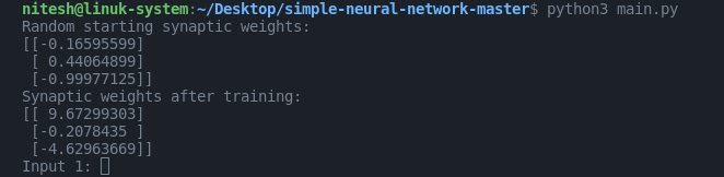
Let’s now take a look at the output of the neural network; Here at the first section, you can see the neural network that assigned itself random weights in the starting section “Random starting synaptic weights:”, then it trained itself using the training set, printing the results in the “Synaptic weights after training:” section.
After that, you can see it’s asking for inputs, which is exactly how we defined it to be in the code and in the start of the article. We can enter it one by one to a total of three, and we should get our results.
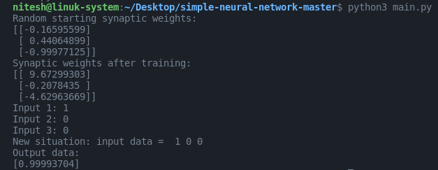
And after entering the values proposed earlier in the article, you can see above we get the output of 0.99993704, which is not exactly the right answer (1) but it’s still very close!
Conclusion
Traditional computer programs do not normally have the capacity for learning. They just do what they’re programmed to do in order to help people get a job done. Much like a calculator helps you with math, but can’t teach itself how to multiply numbers on its own because it doesn’t learn from experience, we can’t rely on traditional programs to resolve the trials and tribulations of the real world by themselves. What’s amazing about neural networks is that they can be creative! They can learn and adapt. Just like the human mind. There are endless possibilities when it comes to neural networks, and equally interesting to create something great or just to learn and play around with.
Here are some useful tutorials that you can read:
- Concurrency in Python
- Instagram bot – posting images, auto like, and bulk follow
- Monitor Python scripts using Prometheus
- Create News Aggregator Site using Python
- Convert an image to 8-bit image
- Create Sudoku game in Python using Pygame
- Get Weather Information using Python
- Create APIs using gRPC in Python
- Pandas Cheat Sheet